---
jupytext:
text_representation:
extension: .md
format_name: myst
format_version: 0.13
jupytext_version: 1.14.7
kernelspec:
display_name: allensdk
language: python
name: allensdk
---
+++ {"papermill": {"duration": 0.009065, "end_time": "2023-03-22T22:19:40.550463", "exception": false, "start_time": "2023-03-22T22:19:40.541398", "status": "completed"}}
# Visual Behavior Neuropixels Quickstart
A short introduction to the Visual Behavior Neuropixels data and SDK. This
notebook focuses on aligning neural data to visual and optotagging stimuli. To
learn more about how to access the data, see our
[data access tutorial](./VBN-Dataset).
For more information about task and behavioral data, check out the
[other tutorials](https://allensdk.readthedocs.io/en/latest/visual_behavior_neuropixels.html)
accompanying this dataset.
Also note that this project shares many features with the
[Visual Coding Neuropixels](http://portal.brain-map.org/explore/circuits/visual-coding-neuropixels)
and
[Visual Behavior 2-Photon](http://portal.brain-map.org/explore/circuits/visual-coding-2p)
datasets. Users are encouraged to check out the documentation for those projects
for additional information and context.
Contents
-------------
* PSTH for image changes
* Plot Receptive Fields
* Optotagging
```{code-cell} ipython3
---
papermill:
duration: 6.299226
end_time: '2023-03-22T22:19:46.856774'
exception: false
start_time: '2023-03-22T22:19:40.557548'
status: completed
---
import os
from pathlib import Path
import numpy as np
import pandas as pd
import matplotlib.pyplot as plt
from allensdk.brain_observatory.behavior.behavior_project_cache.\
behavior_neuropixels_project_cache \
import VisualBehaviorNeuropixelsProjectCache
%matplotlib inline
```
+++ {"papermill": {"duration": 0.006768, "end_time": "2023-03-22T22:19:46.870733", "exception": false, "start_time": "2023-03-22T22:19:46.863965", "status": "completed"}}
The `VisualBehaviorNeuropixelsProjectCache` is the main entry point to the Visual Behavior Neuropixels dataset. It allows you to download data for individual recording sessions and view cross-session summary information.
```{code-cell} ipython3
---
papermill:
duration: 0.015408
end_time: '2023-03-22T22:19:46.892781'
exception: false
start_time: '2023-03-22T22:19:46.877373'
status: completed
tags: [parameters]
---
# Update this to a valid directory in your filesystem. This is where the data will be stored.
cache_dir = '/root/capsule/data/'
cache = VisualBehaviorNeuropixelsProjectCache.from_local_cache(
cache_dir=cache_dir, use_static_cache=True)
```
```{code-cell} ipython3
---
papermill:
duration: 8.864344
end_time: '2023-03-22T22:19:55.784637'
exception: false
start_time: '2023-03-22T22:19:46.920293'
status: completed
---
# get the metadata tables
units_table = cache.get_unit_table()
channels_table = cache.get_channel_table()
probes_table = cache.get_probe_table()
behavior_sessions_table = cache.get_behavior_session_table()
ecephys_sessions_table = cache.get_ecephys_session_table()
```
+++ {"papermill": {"duration": 0.010521, "end_time": "2023-03-22T22:19:55.808215", "exception": false, "start_time": "2023-03-22T22:19:55.797694", "status": "completed"}}
This dataset contains ephys recording sessions from 3 genotypes (C57BL6J, VIP-IRES-CrexAi32 and SST-IRES-CrexAi32). For each mouse, two recordings were made on consecutive days. One of these sessions used the image set that was familiar to the mouse from training. The other session used a novel image set containing two familiar images from training and six new images that the mouse had never seen. As an example, let's grab a session from an SST mouse during a novel session.
```{code-cell} ipython3
---
papermill:
duration: 0.041574
end_time: '2023-03-22T22:19:55.859165'
exception: false
start_time: '2023-03-22T22:19:55.817591'
status: completed
---
sst_novel_sessions = ecephys_sessions_table.loc[(ecephys_sessions_table['genotype'].str.contains('Sst')) &
(ecephys_sessions_table['experience_level']=='Novel')]
sst_novel_sessions.head()
```
+++ {"papermill": {"duration": 0.009862, "end_time": "2023-03-22T22:19:55.879824", "exception": false, "start_time": "2023-03-22T22:19:55.869962", "status": "completed"}}
Now let's choose one of these sessions to look at more closely.
```{code-cell} ipython3
---
papermill:
duration: 143.623875
end_time: '2023-03-22T22:22:19.513449'
exception: false
start_time: '2023-03-22T22:19:55.889574'
status: completed
---
session_id = 1064644573
session = cache.get_ecephys_session(
ecephys_session_id=session_id)
```
+++ {"papermill": {"duration": 0.047743, "end_time": "2023-03-22T22:22:19.652809", "exception": false, "start_time": "2023-03-22T22:22:19.605066", "status": "completed"}}
We can get a high-level summary of this session by accessing its `metadata` attribute:
```{code-cell} ipython3
---
papermill:
duration: 0.06734
end_time: '2023-03-22T22:22:19.767153'
exception: false
start_time: '2023-03-22T22:22:19.699813'
status: completed
---
session.metadata
```
+++ {"papermill": {"duration": 0.046194, "end_time": "2023-03-22T22:22:19.860441", "exception": false, "start_time": "2023-03-22T22:22:19.814247", "status": "completed"}}
Now we can get the unit and channel data for this session. Merging these dataframes will give us CCF coordinates for each unit
```{code-cell} ipython3
---
papermill:
duration: 0.507362
end_time: '2023-03-22T22:22:20.413644'
exception: false
start_time: '2023-03-22T22:22:19.906282'
status: completed
---
units = session.get_units()
channels = session.get_channels()
unit_channels = units.merge(channels, left_on='peak_channel_id', right_index=True)
```
+++ {"papermill": {"duration": 0.047083, "end_time": "2023-03-22T22:22:20.510585", "exception": false, "start_time": "2023-03-22T22:22:20.463502", "status": "completed"}}
Let's look at which brain structures were recorded during this session
```{code-cell} ipython3
---
papermill:
duration: 0.063065
end_time: '2023-03-22T22:22:20.620009'
exception: false
start_time: '2023-03-22T22:22:20.556944'
status: completed
---
unit_channels.value_counts('structure_acronym')
```
+++ {"papermill": {"duration": 0.046545, "end_time": "2023-03-22T22:22:20.714317", "exception": false, "start_time": "2023-03-22T22:22:20.667772", "status": "completed"}}
### PSTH for image changes
+++ {"papermill": {"duration": 0.046021, "end_time": "2023-03-22T22:22:20.807258", "exception": false, "start_time": "2023-03-22T22:22:20.761237", "status": "completed"}}
Now we'll grab spike times and calculate the change response for 'good' units in V1. Note that how you filter units will depend on your analysis. Consult the [unit metrics notebook](https://allensdk.readthedocs.io/en/latest/_static/examples/nb/visual_behavior_neuropixels_quality_metrics.html) for more details.
```{code-cell} ipython3
---
papermill:
duration: 0.067054
end_time: '2023-03-22T22:22:20.920499'
exception: false
start_time: '2023-03-22T22:22:20.853445'
status: completed
---
#first let's sort our units by depth
unit_channels = unit_channels.sort_values('probe_vertical_position', ascending=False)
#now we'll filter them
good_unit_filter = ((unit_channels['snr']>1)&
(unit_channels['isi_violations']<1)&
(unit_channels['firing_rate']>0.1))
good_units = unit_channels.loc[good_unit_filter]
spike_times = session.spike_times
```
+++ {"papermill": {"duration": 0.04651, "end_time": "2023-03-22T22:22:21.013447", "exception": false, "start_time": "2023-03-22T22:22:20.966937", "status": "completed"}}
We can get the times when the image changes occurred from the stimulus presentations table. For now, we'll only take the image changes shown during the active behavior block
```{code-cell} ipython3
---
papermill:
duration: 1.060693
end_time: '2023-03-22T22:22:22.120210'
exception: false
start_time: '2023-03-22T22:22:21.059517'
status: completed
---
stimulus_presentations = session.stimulus_presentations
change_times = stimulus_presentations[stimulus_presentations['active']&
stimulus_presentations['is_change']]['start_time'].values
```
```{code-cell} ipython3
---
papermill:
duration: 0.064425
end_time: '2023-03-22T22:22:22.234380'
exception: false
start_time: '2023-03-22T22:22:22.169955'
status: completed
---
#Convenience function to compute the PSTH
def makePSTH(spikes, startTimes, windowDur, binSize=0.001):
bins = np.arange(0,windowDur+binSize,binSize)
counts = np.zeros(bins.size-1)
for i,start in enumerate(startTimes):
startInd = np.searchsorted(spikes, start)
endInd = np.searchsorted(spikes, start+windowDur)
counts = counts + np.histogram(spikes[startInd:endInd]-start, bins)[0]
counts = counts/startTimes.size
return counts/binSize, bins
```
+++ {"papermill": {"duration": 0.046096, "end_time": "2023-03-22T22:22:22.327109", "exception": false, "start_time": "2023-03-22T22:22:22.281013", "status": "completed"}}
We'll include enough time in our plot to see three image responses: the pre-change image response, the change response and the post-change response
```{code-cell} ipython3
---
papermill:
duration: 0.964636
end_time: '2023-03-22T22:22:23.338269'
exception: false
start_time: '2023-03-22T22:22:22.373633'
status: completed
---
#Here's where we loop through the units in our area of interest and compute their PSTHs
area_of_interest = 'VISp'
area_change_responses = []
area_units = good_units[good_units['structure_acronym']==area_of_interest]
time_before_change = 1
duration = 2.5
for iu, unit in area_units.iterrows():
unit_spike_times = spike_times[iu]
unit_change_response, bins = makePSTH(unit_spike_times,
change_times-time_before_change,
duration, binSize=0.01)
area_change_responses.append(unit_change_response)
area_change_responses = np.array(area_change_responses)
```
```{code-cell} ipython3
---
papermill:
duration: 0.418761
end_time: '2023-03-22T22:22:23.804730'
exception: false
start_time: '2023-03-22T22:22:23.385969'
status: completed
---
#Plot the results
fig, ax = plt.subplots(1,2)
fig.set_size_inches([12,4])
clims = [np.percentile(area_change_responses, p) for p in (0.1,99.9)]
im = ax[0].imshow(area_change_responses, clim=clims)
ax[0].set_title('Active Change Responses for {}'.format(area_of_interest))
ax[0].set_ylabel('Unit number, sorted by depth')
ax[0].set_xlabel('Time from change (s)')
ax[0].set_xticks(np.arange(0, bins.size-1, 20))
_ = ax[0].set_xticklabels(np.round(bins[:-1:20]-time_before_change, 2))
ax[1].plot(bins[:-1]-time_before_change, np.mean(area_change_responses, axis=0), 'k')
ax[1].set_title('{} population active change response (n={})'\
.format(area_of_interest, area_change_responses.shape[0]))
ax[1].set_xlabel('Time from change (s)')
ax[1].set_ylabel('Firing Rate')
```
+++ {"papermill": {"duration": 0.0486, "end_time": "2023-03-22T22:22:23.906718", "exception": false, "start_time": "2023-03-22T22:22:23.858118", "status": "completed"}}
### Plot Receptive Fields
+++ {"papermill": {"duration": 0.049055, "end_time": "2023-03-22T22:22:24.004236", "exception": false, "start_time": "2023-03-22T22:22:23.955181", "status": "completed"}}
Now we'll plot receptive fields for these same units. First we need to get stimulus presentation data for the receptive field mapping stimulus (gabors). For more information about this stimulus, consult [this tutorial](https://allensdk.readthedocs.io/en/latest/_static/examples/nb/ecephys_receptive_fields.html) for the Visual Coding Neuropixels dataset (though note that not all the functionality in the visual coding SDK will work for this dataset).
```{code-cell} ipython3
---
papermill:
duration: 0.067808
end_time: '2023-03-22T22:22:24.120774'
exception: false
start_time: '2023-03-22T22:22:24.052966'
status: completed
---
rf_stim_table = stimulus_presentations[stimulus_presentations['stimulus_name'].str.contains('gabor')]
xs = np.sort(rf_stim_table.position_x.unique()) #positions of gabor along azimuth
ys = np.sort(rf_stim_table.position_y.unique()) #positions of gabor along elevation
```
```{code-cell} ipython3
---
papermill:
duration: 17.592255
end_time: '2023-03-22T22:22:41.762215'
exception: false
start_time: '2023-03-22T22:22:24.169960'
status: completed
---
def find_rf(spikes, xs, ys):
unit_rf = np.zeros([ys.size, xs.size])
for ix, x in enumerate(xs):
for iy, y in enumerate(ys):
stim_times = rf_stim_table[(rf_stim_table.position_x==x)
&(rf_stim_table.position_y==y)]['start_time'].values
unit_response, bins = makePSTH(spikes,
stim_times+0.01,
0.2, binSize=0.001)
unit_rf[iy, ix] = unit_response.mean()
return unit_rf
area_rfs = []
for iu, unit in area_units.iterrows():
unit_spike_times = spike_times[iu]
unit_rf = find_rf(unit_spike_times, xs, ys)
area_rfs.append(unit_rf)
```
```{code-cell} ipython3
---
papermill:
duration: 2.419676
end_time: '2023-03-22T22:22:44.232477'
exception: false
start_time: '2023-03-22T22:22:41.812801'
status: completed
---
fig, axes = plt.subplots(int(len(area_rfs)/10)+1, 10)
fig.set_size_inches(12, 8)
for irf, rf in enumerate(area_rfs):
ax_row = int(irf/10)
ax_col = irf%10
axes[ax_row][ax_col].imshow(rf, origin='lower')
for ax in axes.flat:
ax.axis('off')
```
+++ {"papermill": {"duration": 0.135195, "end_time": "2023-03-22T22:22:44.419665", "exception": false, "start_time": "2023-03-22T22:22:44.284470", "status": "completed"}}
### Optotagging
+++ {"papermill": {"duration": 0.04951, "end_time": "2023-03-22T22:22:44.519137", "exception": false, "start_time": "2023-03-22T22:22:44.469627", "status": "completed"}}
Since this is an SST mouse, we should see putative SST+ interneurons that are activated during our optotagging protocol. Let's load the optotagging stimulus table and plot PSTHs triggered on the laser onset. For more examples and useful info about optotagging, you can check out the Visual Coding Neuropixels Optotagging notebook [here](https://allensdk.readthedocs.io/en/latest/visual_coding_neuropixels.html) (though note that not all the functionality in the visual coding SDK will work for this dataset).
```{code-cell} ipython3
---
papermill:
duration: 0.065743
end_time: '2023-03-22T22:22:44.634261'
exception: false
start_time: '2023-03-22T22:22:44.568518'
status: completed
---
opto_table = session.optotagging_table
opto_table.head()
```
+++ {"papermill": {"duration": 0.050205, "end_time": "2023-03-22T22:22:44.733975", "exception": false, "start_time": "2023-03-22T22:22:44.683770", "status": "completed"}}
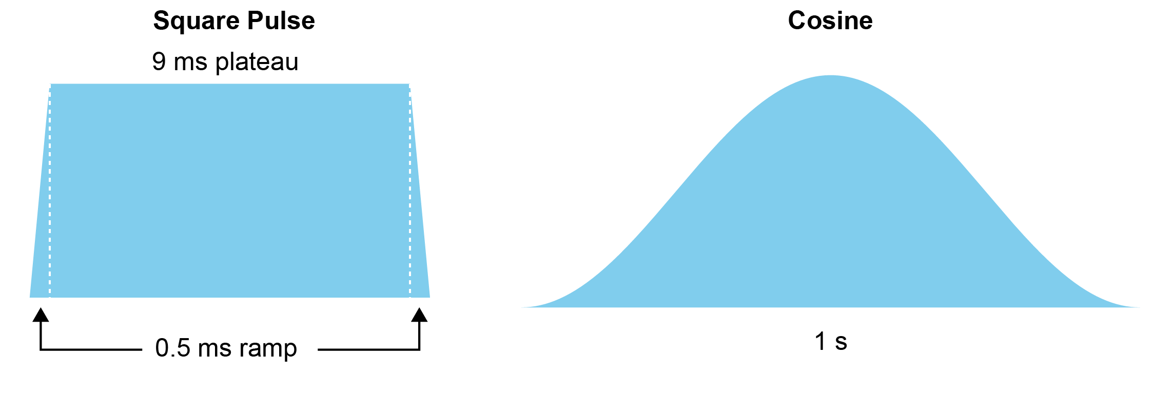
If you check out this table, you'll see that we use 2 different laser waveforms: a short square pulse that's 10 ms long and a half-period cosine that's 1 second long:
+++ {"papermill": {"duration": 0.049513, "end_time": "2023-03-22T22:22:44.832947", "exception": false, "start_time": "2023-03-22T22:22:44.783434", "status": "completed"}}
+++ {"papermill": {"duration": 0.049279, "end_time": "2023-03-22T22:22:44.931901", "exception": false, "start_time": "2023-03-22T22:22:44.882622", "status": "completed"}}
We drive each at three light levels, giving us 6 total conditions. Now let's plot how cortical neurons respond to the short pulse at high power.
```{code-cell} ipython3
---
papermill:
duration: 1.14068
end_time: '2023-03-22T22:22:46.122010'
exception: false
start_time: '2023-03-22T22:22:44.981330'
status: completed
---
duration = opto_table.duration.min() #get the short pulses
level = opto_table.level.max() #and the high power trials
cortical_units = good_units[good_units['structure_acronym'].str.contains('VIS')]
opto_times = opto_table.loc[(opto_table['duration']==duration)&
(opto_table['level']==level)]['start_time'].values
time_before = 0.01 # seconds to take before the laser start for PSTH
duration = 0.03 # total duration of trial for PSTH in seconds
binSize = 0.001 # 1ms bin size for PSTH
opto_response = []
unit_id = []
for iu, unit in cortical_units.iterrows():
unit_spike_times = spike_times[iu]
unit_response, bins = makePSTH(unit_spike_times,
opto_times-time_before, duration,
binSize=binSize)
opto_response.append(unit_response)
unit_id.append(iu)
opto_response = np.array(opto_response)
```
```{code-cell} ipython3
---
papermill:
duration: 0.269406
end_time: '2023-03-22T22:22:46.444435'
exception: false
start_time: '2023-03-22T22:22:46.175029'
status: completed
---
fig, ax = plt.subplots()
fig.set_size_inches((5,10))
fig.suptitle('Optotagging: ' + str(session.metadata['ecephys_session_id'])
+ ' ' + session.metadata['full_genotype'])
im = ax.imshow(opto_response,
origin='lower', aspect='auto',
)
min_clim_val = 0
max_clim_val = 250
im.set_clim([min_clim_val, max_clim_val])
[ax.axvline(bound, linestyle=':', color='white', linewidth=1.0)\
for bound in [10, 19]]
ax.set_xlabel('Time from laser onset (ms)')
ax.set_ylabel('Unit number')
ax.set_xticks(1000*bins[:-1:5])
time_labels = np.round(1000*(bins[:-1:5]-time_before), 0)
_=ax.set_xticklabels(time_labels)
```
+++ {"papermill": {"duration": 0.052442, "end_time": "2023-03-22T22:22:46.555721", "exception": false, "start_time": "2023-03-22T22:22:46.503279", "status": "completed"}}
Here we can see that most units don't respond to the short laser pulse. But there is a population that do show elevated firing rates. Note that the activity occurring at the onset and offset of the laser (along the dotted lines) is artifactual and should be excluded from analysis.
Let's plot the response to the laser over the population:
```{code-cell} ipython3
---
papermill:
duration: 0.061302
end_time: '2023-03-22T22:22:46.669822'
exception: false
start_time: '2023-03-22T22:22:46.608520'
status: completed
---
baseline_window = slice(0, 9) # baseline epoch
response_window = slice(11,18) # laser epoch
response_magnitudes = np.mean(opto_response[:, response_window], axis=1) \
- np.mean(opto_response[:, baseline_window], axis=1)
```
```{code-cell} ipython3
---
papermill:
duration: 0.570857
end_time: '2023-03-22T22:22:47.293100'
exception: false
start_time: '2023-03-22T22:22:46.722243'
status: completed
---
fig, axes = plt.subplots(1,2)
fig.set_size_inches(10, 5)
# Plot scatter of opto rate vs baseline rate
axes[0].plot(np.mean(opto_response[:, baseline_window], axis=1),
np.mean(opto_response[:, response_window], axis=1), 'k.', alpha=0.2)
axes[0].set_xlim([-10, 200])
axes[0].set_ylim([-10, 400])
axes[0].set_aspect('equal')
axes[0].set_ylabel('response rate (Hz)')
axes[0].set_xlabel('baseline rate (Hz)')
# Plot histogram of opto-evoked rate (note log yscale)
_ = axes[1].hist(response_magnitudes, bins=20)
axes[1].set_yscale('log')
axes[1].set_xlabel('Opto-evoked rate (Hz)')
axes[1].set_ylabel('Unit Count')
```